Dynamic Programming Patterns

Pattern Classification

Recognising which DP pattern applies to a problem is the key skill. This section provides a decision Framework.

Decision Tree

Signal	Pattern	Example
Choose items with capacity constraint	Knapsack	0/1 knapsack, subset sum
Optimise over intervals/substrings	Interval DP	Matrix chain, burst balloons
Problem on a tree structure	Tree DP	Diameter, independent set
Small set of items (n <= 20)	Bitmask DP	TSP, assignment
Count numbers with digit properties	Digit DP	Numbers with no “4’ and ‘7’
Optimise over subsequences/strings	String DP	Edit distance, LCS
Two players taking turns	Game theory DP	Nim, coin game
Greedy seems to work	Greedy-reducible DP	Activity selection

Knapsack Family

0/1 Knapsack

Given $n$ items with weights $w_i$ and values $v_i$ And a knapsack of capacity $W$ Maximise the Total value of items selected. Each item can be taken at most once.

$dp[i][c] = \max(dp[i-1][c], dp[i-1][c - w_i] + v_i) \quad \mathrm{if c \ge w_i$

def knapsack_01(weights, values, capacity):
    """
    0/1 knapsack — each item used at most once.
    Time: O(n * W)
    Space: O(W) with 1D optimisation
    """
    n = len(weights)
    dp = [0] * (capacity + 1)

    for i in range(n):
        w, v = weights[i], values[i]
        for c in range(capacity, w - 1, -1):
            dp[c] = max(dp[c], dp[c - w] + v)

    return dp[capacity]

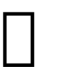
Iterate forward, `dp[c - w]` may already include item $i$Violating the 0/1 constraint. This is the Most common bug in knapsack implementations.

Unbounded Knapsack

Each item can be taken unlimited times. Iterate capacity forward.

def knapsack_unbounded(weights, values, capacity):
    """
    Unbounded knapsack — items can be reused.
    Time: O(n * W)
    Space: O(W)
    """
    dp = [0] * (capacity + 1)
    for c in range(1, capacity + 1):
        for w, v in zip(weights, values):
            if w <= c:
                dp[c] = max(dp[c], dp[c - w] + v)
    return dp[capacity]

Bounded Knapsack

Each item can be taken at most $k_i$ times. Convert to 0/1 knapsack by binary decomposition.

def knapsack_bounded(weights, values, counts, capacity):
    """
    Bounded knapsack — each item has a maximum count.
    Uses binary decomposition to convert to 0/1 knapsack.
    Time: O(W * sum(log k_i))
    Space: O(W)
    """
    expanded_w, expanded_v = [], []
    for w, v, k in zip(weights, values, counts):
        amt = k
        power = 1
        while power <= amt:
            expanded_w.append(w * power)
            expanded_v.append(v * power)
            amt -= power
            power *= 2
        if amt > 0:
            expanded_w.append(w * amt)
            expanded_v.append(v * amt)
    return knapsack_01(expanded_w, expanded_v, capacity)

Subset Sum

Given a set of integers, determine if a subset sums to a target.

def subset_sum(nums, target):
    """
    Check if any subset sums to target.
    Time: O(n * target)
    Space: O(target)
    """
    dp = [False] * (target + 1)
    dp[0] = True
    for num in nums:
        for t in range(target, num - 1, -1):
            dp[t] = dp[t] or dp[t - num]
    return dp[target]

Partition Equal Subset Sum

def can_partition(nums):
    """
    Check if array can be partitioned into two equal-sum subsets.
    Time: O(n * sum(nums) / 2)
    Space: O(sum(nums) / 2)
    """
    total = sum(nums)
    if total % 2 != 0:
        return False
    return subset_sum(nums, total // 2)

Multi-Dimensional Knapsack

When there are multiple constraints (e.g., weight and volume), the DP state has multiple dimensions.

def knapsack_2d(weights, volumes, values, max_weight, max_volume):
    """
    2D knapsack with weight and volume constraints.
    Time: O(n * max_weight * max_volume)
    Space: O(max_weight * max_volume)
    """
    dp = [[0] * (max_volume + 1) for _ in range(max_weight + 1)]
    for w, v, val in zip(weights, volumes, values):
        for c in range(max_weight, w - 1, -1):
            for d in range(max_volume, v - 1, -1):
                dp[c][d] = max(dp[c][d], dp[c - w][d - v] + val)
    return dp[max_weight][max_volume]

Interval DP

Interval DP solves problems on contiguous subarrays/substrings by considering all possible Partitions of an interval.

Matrix Chain Multiplication

Given matrices $A_1, A_2, \ldots, A_n$ where $A_i$ has dimensions $p_{i-1} \times p_i$ Find the Parenthesisation that minimises the total number of scalar multiplications.

$dp[i][j] = \min_{i \le k \lt j} (dp[i][k] + dp[k+1][j] + p_{i-1} \cdot p_k \cdot p_j)$

def matrix_chain_order(p):
    """
    Optimal parenthesisation of matrix chain multiplication.
    Time: O(n^3)
    Space: O(n^2)
    """
    n = len(p) - 1
    dp = [[0] * (n + 1) for _ in range(n + 1)]
    split = [[0] * (n + 1) for _ in range(n + 1)]

    for length in range(2, n + 1):
        for i in range(1, n - length + 2):
            j = i + length - 1
            dp[i][j] = float('inf')
            for k in range(i, j):
                cost = dp[i][k] + dp[k + 1][j] + p[i - 1] * p[k] * p[j]
                if cost < dp[i][j]:
                    dp[i][j] = cost
                    split[i][j] = k

    def build_parenthesis(i, j):
        if i == j:
            return f"A{i}"
        return f"({build_parenthesis(i, split[i][j])} x {build_parenthesis(split[i][j] + 1, j)})"

    return dp[1][n], build_parenthesis(1, n)

Burst Balloons

Given numsWhere nums[i] is the value of the $i$ -th balloon, bursting balloon $i$ yields nums[left] * nums[i] * nums[right] coins where left and right are the adjacent unburst Balloons. Maximise total coins.

def burst_balloons(nums):
    """
    Maximize coins from bursting balloons.
    Time: O(n^3)
    Space: O(n^2)
    Key insight: think about which balloon to burst LAST, not first.
    """
    n = len(nums)
    padded = [1] + nums + [1]
    dp = [[0] * (n + 2) for _ in range(n + 2)]

    for length in range(1, n + 1):
        for left in range(1, n - length + 2):
            right = left + length - 1
            for k in range(left, right + 1):
                coins = padded[left - 1] * padded[k] * padded[right + 1]
                dp[left][right] = max(
                    dp[left][right],
                    dp[left][k - 1] + coins + dp[k + 1][right]
                )

    return dp[1][n]

Minimum Cost to Merge Stones

Given $n$ piles of stones and an integer $k$ Merge adjacent piles into one pile. Each merge of $k$ Piles costs the sum of those $k$ piles. Find the minimum total cost, or return -1 if impossible.

def merge_stones(stones, k):
    """
    Minimum cost to merge stones with exactly k piles per merge.
    Time: O(n^3 / k)
    Space: O(n^2)
    Possible iff (n - 1) % (k - 1) == 0
    """
    n = len(stones)
    if (n - 1) % (k - 1) != 0:
        return -1

    prefix = [0] * (n + 1)
    for i in range(n):
        prefix[i + 1] = prefix[i] + stones[i]

    dp = [[0] * n for _ in range(n)]

    for length in range(k, n + 1):
        for i in range(n - length + 1):
            j = i + length - 1
            dp[i][j] = float('inf')
            for m in range(i, j, k - 1):
                dp[i][j] = min(dp[i][j], dp[i][m] + dp[m + 1][j])
            if (j - i) % (k - 1) == 0:
                dp[i][j] += prefix[j + 1] - prefix[i]

    return dp[0][n - 1]

Interval DP Template

def interval_dp_template(arr):
    """
    Generic interval DP template.
    Time: O(n^3) or O(n^2) depending on transition
    Space: O(n^2)
    """
    n = len(arr)
    dp = [[0] * n for _ in range(n)]

    for length in range(2, n + 1):
        for left in range(n - length + 1):
            right = left + length - 1
            for mid in range(left, right):
                dp[left][right] = min(
                    dp[left][right],
                    dp[left][mid] + dp[mid + 1][right] + cost(left, mid, right)
                )

    return dp[0][n - 1]

Tree DP

Tree DP applies dynamic programming on tree structures, using post-order traversal (process children before parent).

Tree Diameter

def tree_diameter(n, edges):
    """
    Diameter of a tree (longest path).
    Time: O(n)
    Space: O(n)
    """
    from collections import defaultdict
    graph = defaultdict(list)
    for u, v in edges:
        graph[u].append(v)
        graph[v].append(u)

    diameter = 0

    def dfs(node, parent):
        nonlocal diameter
        max1 = max2 = 0
        for neighbor in graph[node]:
            if neighbor == parent:
                continue
            depth = dfs(neighbor, node)
            if depth > max1:
                max2 = max1
                max1 = depth
            elif depth > max2:
                max2 = depth
        diameter = max(diameter, max1 + max2)
        return max1 + 1

    dfs(0, -1)
    return diameter

Maximum Path Sum on Binary Tree

def max_path_sum(root):
    """
    Maximum path sum in a binary tree.
    A path is any node-to-node sequence (not necessarily through root).
    Time: O(n)
    Space: O(h) recursion stack
    """
    result = float('-inf')

    def dfs(node):
        nonlocal result
        if node is None:
            return 0
        left = max(0, dfs(node.left))
        right = max(0, dfs(node.right))
        result = max(result, node.val + left + right)
        return node.val + max(left, right)

    dfs(root)
    return result

Maximum Independent Set on Trees

def max_independent_set(n, edges):
    """
    Maximum independent set on a tree.
    An independent set has no two adjacent nodes.
    Time: O(n)
    Space: O(n)
    """
    from collections import defaultdict
    graph = defaultdict(list)
    for u, v in edges:
        graph[u].append(v)
        graph[v].append(u)

    def dfs(node, parent):
        include = 1
        exclude = 0
        for neighbor in graph[node]:
            if neighbor == parent:
                continue
            child_inc, child_exc = dfs(neighbor, node)
            include += child_exc
            exclude += max(child_inc, child_exc)
        return include, exclude

    return max(dfs(0, -1))

Tree DP with Rerooting

Rerooting solves the problem: compute some property for every node as the root.

def rerooting_dp(n, edges):
    """
    Compute DP value for every node as root.
    Time: O(n)
    Space: O(n)
    """
    from collections import defaultdict, deque
    graph = defaultdict(list)
    for u, v, w in edges:
        graph[u].append((v, w))
        graph[v].append((u, w))

    parent = [0] * n
    children = [[] for _ in range(n)]
    order = []
    stack = [0]
    visited = [False] * n
    visited[0] = True

    while stack:
        node = stack.pop()
        order.append(node)
        for neighbor, w in graph[node]:
            if not visited[neighbor]:
                visited[neighbor] = True
                parent[neighbor] = node
                children[node].append((neighbor, w))
                stack.append(neighbor)

    down = [0] * n
    for node in reversed(order):
        for child, w in children[node]:
            down[node] += down[child] + w

    up = [0] * n
    for node in order:
        total_children = sum(down[c] + w for c, w in children[node])
        for child, w in children[node]:
            up[child] = up[node] + (total_children - (down[child] + w))

    result = [down[i] + up[i] for i in range(n)]
    return result

Bitmask DP

Bitmask DP uses bitmasks to represent subsets, enabling $O(2^n \cdot n)$ solutions for problems with Small $n$ ( $n \le 20$ ).

Travelling Salesman Problem (TSP)

Find the shortest Hamiltonian cycle visiting all cities exactly once.

$dp[mask][i] = \min_{j \in mask, j \ne i} (dp[mask \setminus \{i\}][j] + dist[j][i])$

def tsp(dist):
    """
    Travelling Salesman Problem.
    Time: O(2^n * n^2)
    Space: O(2^n * n)
    n must be small (in standard practice n <= 20).
    """
    n = len(dist)
    full_mask = (1 << n) - 1
    INF = float('inf')
    dp = [[INF] * n for _ in range(1 << n)]
    dp[1][0] = 0

    for mask in range(1, 1 << n):
        for u in range(n):
            if not (mask & (1 << u)):
                continue
            if dp[mask][u] == INF:
                continue
            for v in range(n):
                if mask & (1 << v):
                    continue
                new_mask = mask | (1 << v)
                dp[new_mask][v] = min(dp[new_mask][v], dp[mask][u] + dist[u][v])

    result = INF
    for u in range(1, n):
        result = min(result, dp[full_mask][u] + dist[u][0])

    return result

Assignment Problem

Assign $n$ workers to $n$ tasks, minimising total cost.

def assignment(cost):
    """
    Minimum cost assignment problem.
    Time: O(2^n * n)
    Space: O(2^n)
    """
    n = len(cost)
    dp = [float('inf')] * (1 << n)
    dp[0] = 0

    for mask in range(1 << n):
        worker = bin(mask).count('1')
        if worker >= n:
            continue
        for task in range(n):
            if not (mask & (1 << task)):
                new_mask = mask | (1 << task)
                dp[new_mask] = min(dp[new_mask], dp[mask] + cost[worker][task])

    return dp[(1 << n) - 1]

Digit DP

Digit DP counts numbers in a range that satisfy certain digit-based properties by processing digits From most significant to least significant.

Template

def digit_dp(lo, hi):
    """
    Count numbers in [lo, hi] satisfying a property.
    Time: O(digits * states * 10)
    Space: O(digits * states)
    """
    def count(n):
        if n < 0:
            return 0
        digits = list(map(int, str(n)))

        def dfs(pos, tight, state):
            if pos == len(digits):
                return 1 if is_valid(state) else 0
            limit = digits[pos] if tight else 9
            total = 0
            for d in range(limit + 1):
                new_state = transition(state, d)
                total += dfs(pos + 1, tight and d == limit, new_state)
            return total

        return dfs(0, True, initial_state())

    return count(hi) - count(lo - 1)

Count Numbers Without Consecutive 1s in Binary

def count_no_consecutive_ones(n):
    """
    Count numbers from 0 to n with no consecutive 1s in binary.
    Time: O(log^2 n)
    """
    def count_limit(n):
        s = bin(n)[2:]
        length = len(s)

        def dfs(pos, tight, prev_one):
            if pos == length:
                return 1
            limit = int(s[pos]) if tight else 1
            total = 0
            for d in range(limit + 1):
                if d == 1 and prev_one:
                    continue
                total += dfs(pos + 1, tight and d == limit, d == 1)
            return total

        return dfs(0, True, False)

    return count_limit(n)

String DP

Edit Distance (Levenshtein Distance)

Minimum number of insertions, deletions, and substitutions to transform one string into another.

$dp[i][j] = \begin{cases} dp[i-1][j-1] & \mathrm{if s[i] = t[j] \\ 1 + \min(dp[i-1][j], dp[i][j-1], dp[i-1][j-1]) & \mathrm{otherwise \end{cases}$

def edit_distance(s, t):
    """
    Levenshtein distance between two strings.
    Time: O(m * n)
    Space: O(min(m, n)) with 1D optimisation
    """
    m, n = len(s), len(t)
    if m < n:
        s, t = t, s
        m, n = n, m

    prev = list(range(n + 1))
    curr = [0] * (n + 1)

    for i in range(1, m + 1):
        curr[0] = i
        for j in range(1, n + 1):
            if s[i - 1] == t[j - 1]:
                curr[j] = prev[j - 1]
            else:
                curr[j] = 1 + min(prev[j], curr[j - 1], prev[j - 1])
        prev, curr = curr, prev

    return prev[n]

Longest Common Subsequence

def lcs(s, t):
    """
    Longest common subsequence.
    Time: O(m * n)
    Space: O(min(m, n))
    """
    m, n = len(s), len(t)
    if m < n:
        s, t = t, s
        m, n = n, m

    prev = [0] * (n + 1)
    for i in range(1, m + 1):
        curr = [0] * (n + 1)
        for j in range(1, n + 1):
            if s[i - 1] == t[j - 1]:
                curr[j] = prev[j - 1] + 1
            else:
                curr[j] = max(prev[j], curr[j - 1])
        prev = curr

    return prev[n]

Longest Palindromic Subsequence

def longest_palindromic_subsequence(s):
    """
    Longest palindromic subsequence.
    Time: O(n^2)
    Space: O(n^2)
    """
    n = len(s)
    dp = [[0] * n for _ in range(n)]
    for i in range(n):
        dp[i][i] = 1
    for length in range(2, n + 1):
        for i in range(n - length + 1):
            j = i + length - 1
            if s[i] == s[j]:
                dp[i][j] = dp[i + 1][j - 1] + 2 if length > 2 else 2
            else:
                dp[i][j] = max(dp[i + 1][j], dp[i][j - 1])
    return dp[0][n - 1]

Regex Matching

def is_match(s, p):
    """
    Regex matching with '.' and '*'.
    Time: O(m * n)
    Space: O(n)
    """
    m, n = len(s), len(p)
    dp = [False] * (n + 1)
    dp[0] = True

    for j in range(2, n + 1):
        if p[j - 1] == '*':
            dp[j] = dp[j - 2]

    for i in range(1, m + 1):
        new_dp = [False] * (n + 1)
        for j in range(1, n + 1):
            if p[j - 1] == '*':
                new_dp[j] = new_dp[j - 2]
                if p[j - 2] == s[i - 1] or p[j - 2] == '.':
                    new_dp[j] = new_dp[j] or dp[j]
            elif p[j - 1] == s[i - 1] or p[j - 1] == '.':
                new_dp[j] = dp[j - 1]
        dp = new_dp

    return dp[n]

Game Theory DP

Nim and Sprague-Grundy Theorem

Every impartial game (where the available moves depend only on the position, not on which player is Moving) is equivalent to a Nim heap. The Sprague-Grundy theorem states that the Grundy number (mex Of children’s Grundy numbers) determines the winning strategy.

def grundy_number(positions):
    """
    Compute Grundy number as mex of reachable positions.
    mex = minimum excluded value.
    """
    reachable = set()
    for move in get_moves(positions):
        reachable.add(grundy_number(move))
    mex = 0
    while mex in reachable:
        mex += 1
    return mex

def nim_winner(heaps):
    """
    Determine winner of Nim game.
    Winner: first player iff XOR of all heaps != 0.
    Time: O(n)
    """
    xor_sum = 0
    for h in heaps:
        xor_sum ^= h
    return xor_sum != 0

Coin Game

def coin_game(coins):
    """
    Two players alternate taking coins from either end.
    Max amount the first player can collect.
    Time: O(n^2)
    Space: O(n^2)
    """
    n = len(coins)
    dp = [[0] * n for _ in range(n)]
    for i in range(n):
        dp[i][i] = coins[i]
    for length in range(2, n + 1):
        for i in range(n - length + 1):
            j = i + length - 1
            dp[i][j] = max(
                coins[i] + min(dp[i + 2][j] if i + 2 <= j else 0,
                               dp[i + 1][j - 1] if i + 1 <= j - 1 else 0),
                coins[j] + min(dp[i + 1][j - 1] if i + 1 <= j - 1 else 0,
                               dp[i][j - 2] if i <= j - 2 else 0)
            )
    return dp[0][n - 1]

Greedy-Reducible DP

Some DP problems have greedy solutions that are simpler and faster. The key question: does making The locally optimal choice always lead to the globally optimal solution?

When Greedy Works Instead of DP

Problem	Greedy Works?	Greedy Strategy
Fractional knapsack	Yes	Sort by value/weight ratio
Activity selection	Yes	Earliest finish time
Huffman coding	Yes	Merge two smallest frequencies
Minimum spanning tree	Yes	Kruskal / Prim
Dijkstra (non-negative)	Yes	Process smallest distance
0/1 knapsack	No	DP required
Partition equal subset sum	No	DP required
Edit distance	No	DP required

State Compression Techniques

Reducing State Space

Technique	When to Use	Example
Coordinate compression	Large coordinate values, few unique	`sorted(set(values))` + binary search
Difference encoding	State depends on differences	`dp[i][diff]` instead of `dp[i][a][b]`
Rolling array	Only previous row/column needed	`prev` and `curr` arrays
Bitmask	Small set of choices (n <= 20)	TSP, assignment
Sparse DP	Many states unreachable	Dictionary instead of array

Common Pitfalls

1. Wrong Iteration Order

The fill order must respect the dependency: if dp[i] depends on dp[j]Then j must be computed Before i. For interval DP, always iterate by increasing interval length. For 1D DP, verify whether Forward or backward iteration is needed (0/1 knapsack needs backward, unbounded needs forward).

2. Integer Overflow in DP Values

DP values can grow exponentially (e.g., counting paths in a grid). Use Python’s arbitrary-precision Integers, or in C++/Java, use long long or BigInteger. Always check whether the problem asks for The result modulo some value.

3. Off-by-One in Bitmask DP

In bitmask DP, mask & (1 << i) tests whether bit $i$ is set. mask | (1 << i) sets bit $i$ . mask & ~(1 << i) clears bit $i$ . Forgetting the parentheses around 1 << i in ~(1 << i) is a Common bug because ~ has lower precedence than &.

4. Forgetting Base Cases

Missing or incorrect base cases are the most common DP bug. For interval DP, the base case is dp[i][i]. For tree DP, the base case is the leaf node. For string DP, the base case is the empty String. Always verify base cases by hand before writing the transition.

5. Confusing Subsequence and Subarray

A subsequence is not necessarily contiguous; a subarray (or substring) is. “Longest increasing Subsequence” uses DP over subsequences ( $O(n^2)$ or $O(n \log n)$ ). “Maximum sum subarray” uses Kadane’s algorithm ( $O(n)$ ). Mixing these up leads to incorrect solutions.

6. Digit DP `tight` Flag Mishandling

In digit DP, the tight flag indicates whether the prefix matches the upper bound. When tight is False, you can use any digit (0-9). When tight is True, you can only use digits up to the current Digit of the upper bound. Forgetting to propagate tight correctly produces wrong counts.

7. Tree DP Root Assumption

Tree DP solutions often assume a specific root ( node 0). If the problem asks for a Property of the tree regardless of root (e.g., diameter), make sure the solution does not depend on The root choice. For problems that require computing a value for every node as root, use rerooting DP.

8. Overcounting in Game Theory DP

In game theory DP, the standard formulation computes the value that the current player can Guarantee. A common mistake is to assume both players play optimally for the same objective. In Zero-sum games, player 1 maximises while player 2 minimises. Getting this wrong inverts the result.

Summary

This topic covers the core concepts of dynamic programming patterns, including underlying theory, practical implementation, and key applications.

Key concepts include:

variables, data types, and control flow
functions and procedures
object-oriented programming
error handling and debugging
modular design

Understanding these concepts thoroughly is essential for both examinations and practical programming, and requires both theoretical knowledge and hands-on practice.

Worked Examples

Worked examples demonstrating the application of key concepts are covered in the detailed sub-pages linked above.

Cross-References

Dynamic Programming: Core DP concepts including memoisation and tabulation that underpin these patterns.
Sorting Algorithms: Sorting techniques often used as preprocessing steps in DP problems.
Hashing and Hash Tables: Hash-based data structures used for memoisation in top-down DP approaches.

Intuition

The fundamental idea behind all DP patterns is the same: break a problem into overlapping subproblems, solve each subproblem once, and reuse the results. What changes between patterns is the shape of the subproblems. Linear DP arranges subproblems in a line (like climbing stairs). Interval DP works on ranges (like matrix chain multiplication). Tree DP traverses a tree structure. Bitmask DP represents subsets as bit patterns. The core skill is recognizing which “shape” your problem has, because that determines how you define states and transitions.

The hardest part of DP is in most cases defining the right state — what information do you need to capture at each subproblem? A good rule of thumb is: the state should contain everything that affects future decisions but nothing redundant. For interval DP, the state is (left, right) because the optimal solution for a range depends only on that range. For tree DP, you process children before parents (post-order) because a node’s optimal value depends on its subtree. For bitmask DP, the bitmask itself is the state — it tells you exactly which elements have been used.

Once you have the right state, the transition is in most cases straightforward: try all possible “last moves” and take the best one. The key to efficiency is recognizing when you can reduce the state space: rolling arrays when you only need the previous row, coordinate compression when values are large but few, and sparse representations when most states are unreachable. And always, always check your base cases by hand before coding — a missing or wrong base case is the most common DP bug.

Mark this page as reviewed