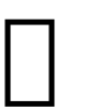
At O ( E + V log V ) O(E + V \log V) O ( E + V log V ) E ≈ V E \approx V E ≈ V
Find all strongly connected components (SCCs) in a directed graph using two DFS passes.
Run DFS on the original graph, pushing vertices onto a stack in order of finishing time Compute the transpose (reverse all edges) Run DFS on the transpose in the order determined by the stack Find strongly connected components using Kosaraju's algorithm.
Time: O(V + E), Space: O(V + E)
Returns list of SCCs (each SCC is a list of vertices).
for neighbour, _ in graph.neighbours(v):
if neighbour not in visited:
transpose = {v: [] for v in graph.adj}
for neighbour, _ in graph.neighbours(v):
transpose[neighbour].append(v)
for v in reversed (order):
for neighbour in transpose[node]:
if neighbour not in visited:
Tarjan’s algorithm finds SCCs in a single DFS pass using a stack and low-link values.
Find SCCs using Tarjan's algorithm.
Time: O(V + E), Space: O(V)
index[v] = index_counter[ 0 ]
lowlink[v] = index_counter[ 0 ]
for neighbour, _ in graph.neighbours(v):
if neighbour not in index:
lowlink[v] = min (lowlink[v], lowlink[neighbour])
elif neighbour in on_stack:
lowlink[v] = min (lowlink[v], index[neighbour])
if lowlink[v] == index[v]:
The Ford-Fulkerson method finds the maximum flow in a flow network by repeatedly finding augmenting Paths from source to sink and pushing flow along them.
def ford_fulkerson ( n , capacity , source , sink ):
Ford-Fulkerson max flow (Edmonds-Karp implementation with BFS).
Time: O(V * E^2) with BFS (Edmonds-Karp)
capacity: adjacency matrix capacity[u][v] = max flow on edge u->v
if not visited[v] and capacity[u][v] > 0 :
# Find minimum residual capacity along the path
path_flow = min (path_flow, capacity[u][v])
# Update residual capacities
capacity[u][v] -= path_flow
capacity[v][u] += path_flow # add reverse edge
Edmonds-Karp is Ford-Fulkerson where the augmenting path is found using BFS (shortest path in terms of number of edges). This guarantees O ( V E 2 ) O(VE^2) O ( V E 2 )
The maximum flow from source to sink equals the minimum capacity of any cut separating source from Sink. A cut is a partition of vertices into two sets S S S T T T S S S T T T
def min_cut ( n , capacity , source , sink ):
Find min cut after computing max flow.
Returns (cut_capacity, s_side, t_side).
# Run Edmonds-Karp to get residual graph
max_flow = ford_fulkerson(n, capacity, source, sink)
# BFS on residual graph to find reachable vertices from source
if not visited[v] and capacity[u][v] > 0 :
s_side = [i for i in range (n) if visited[i]]
t_side = [i for i in range (n) if not visited[i]]
return max_flow, s_side, t_side
Application How to Model Bipartite matching Source to left set, right set to sink, all edges capacity 1 Image segmentation Pixels as vertices, source=foreground, sink=background Project selection Source=projects, sink=resources, capacities=profits/costs Baseball elimination Teams as vertices, remaining games as edges Network reliability Edge connectivity via min-cut
An Eulerian circuit visits every edge exactly once and returns to the start. An Eulerian Path visits every edge exactly once (may start and end at different vertices).
Property Eulerian Circuit Eulerian Path Connected Yes Yes All vertices even degree Yes No Exactly 2 vertices odd degree No Yes (start/end at odd vertices) Other No No
def hierholzer ( n , graph ):
Find Eulerian circuit using Hierholzer's algorithm.
Time: O(V + E), Space: O(V + E)
Assumes Eulerian circuit exists.
adj = {v: list (neighbours) for v, neighbours in graph.items()}
circuit.append(stack.pop())
A graph is bipartite if and only if it is 2-colorable. Use BFS to assign colors.
The chromatic number χ ( G ) \chi(G) χ ( G )
def greedy_coloring ( n , graph ):
Time: O(V + E), Space: O(V)
Uses at most max_degree + 1 colors (by Brook's theorem, at most max_degree for connected graphs
that are not complete or odd cycles).
for neighbour in graph.get(v, []):
if colors[neighbour] != - 1 :
used.add(colors[neighbour])
# Find smallest available color
Brook’s Theorem: For a connected graph that is neither a complete graph nor an odd cycle, χ ( G ) ≤ Δ ( G ) \chi(G) \le \Delta(G) χ ( G ) ≤ Δ ( G ) Δ ( G ) \Delta(G) Δ ( G ) Δ + 1 \Delta + 1 Δ + 1 Δ \Delta Δ
Given a complete graph with weighted edges, find the Hamiltonian cycle of minimum total weight. TSP is NP-hard; exact solutions use bitmask DP (O ( 2 n ⋅ n 2 ) O(2^n \cdot n^2) O ( 2 n ⋅ n 2 ) n ≤ 20 n \le 20 n ≤ 20
Algorithm Approximation Ratio Time Notes Nearest neighbour O ( log n ) O(\log n) O ( log n ) O ( n 2 ) O(n^2) O ( n 2 ) Simple, no guarantee Christofides 1.5 O ( n 3 ) O(n^3) O ( n 3 ) Best known for metric TSP 2-opt improvement Empirical O ( n 2 ) O(n^2) O ( n 2 ) Local search Held-Karp (DP) Exact O ( 2 n ⋅ n 2 ) O(2^n \cdot n^2) O ( 2 n ⋅ n 2 ) Exact, n ≤ 20 n \le 20 n ≤ 20
Metric TSP: When the triangle inequality holds (d ( u , w ) ≤ d ( u , v ) + d ( v , w ) d(u, w) \le d(u, v) + d(v, w) d ( u , w ) ≤ d ( u , v ) + d ( v , w )
def tsp_nearest_neighbour ( dist ):
Nearest neighbour heuristic for TSP.
No approximation guarantee, but often reasonable in practice.
nearest_dist = float ( ' inf ' )
if not visited[j] and dist[current][j] < nearest_dist:
nearest_dist = dist[current][j]
total += dist[path[ - 1 ]][path[ 0 ]] # return to start
Single source, non-negative weights: DijkstraSingle source, negative weights: Bellman-FordAll pairs, small V: Floyd-WarshallAll pairs, large V, sparse: Run Dijkstra V V V With heuristic: A*Unweighted: BFSKahn’s algorithm (BFS): Process vertices with in-degree 0DFS-based: Process in reverse post-orderApplication: Build systems (Make), course scheduling, deadlock detectionUndirected: BFS/DFS from each unvisited vertexStrongly connected (directed): Kosaraju’s or Tarjan’s algorithmApplication: Social network communities, image segmentationSparse graph: Kruskal’s with Union-FindDense graph: Prim’s with priority queueApplication: Network design, clusteringMax flow: Ford-Fulkerson / Edmonds-KarpMin cut: Complement of max flowBipartite matching: Max flow with unit capacitiesApplication: Matching, assignment, schedulingDijkstra does not work with negative edge weights. The algorithm assumes that processing a vertex Means its shortest distance is final, but a negative edge can provide a shorter path to an already- Processed vertex. Use Bellman-Ford for graphs with negative weights.
In Floyd-Warshall, the relaxation step is dist[i][j] = min(dist[i][j], dist[i][k] + dist[k][j]). If dist[i][k] or dist[k][j] is infThe sum becomes infWhich is correct. But if your inf Is not large enough (e.g., float('inf') / 2 + float('inf') / 2), you may get incorrect results. Use a sufficiently large sentinel value or handle infinity explicitly.
Without path compression, Kruskal’s Union-Find operations degrade to O ( log n ) O(\log n) O ( log n ) O ( E log V + E log V ) = O ( E log V ) O(E \log V + E \log V) = O(E \log V) O ( E log V + E log V ) = O ( E log V ) O ( E ⋅ α ( V ) ) O(E \cdot \alpha(V)) O ( E ⋅ α ( V )) O ( E ) O(E) O ( E )
If the heuristic overestimates the true distance, A* is not guaranteed to find the shortest path. It may still find a path quickly, but it will be suboptimal. For pathfinding in games, this is often Acceptable (speed over optimality). For navigation systems, it is not.
Kruskal’s and Prim’s algorithms assume a connected graph. If the graph is disconnected, they will Produce a minimum spanning forest (one tree per connected component). If you need to detect Disconnection, check that the MST has V − 1 V - 1 V − 1
Using list.pop(0) for BFS is O ( n ) O(n) O ( n ) O ( n 2 ) O(n^2) O ( n 2 ) collections.deque With popleft() for O ( 1 ) O(1) O ( 1 )
Modifying the graph structure (adding/removing vertices or edges) during BFS/DFS traversal leads to Undefined behaviour, vertices may be skipped or processed multiple times. If you need to modify the Graph, collect the modifications and apply them after the traversal completes.
Ford-Fulkerson may not terminate with irrational capacities (the flow can converge without reaching the maximum). Edmonds-Karp (BFS-based) always terminates with O ( V E 2 ) O(VE^2) O ( V E 2 ) O ( E ⋅ f ∗ ) O(E \cdot f^*) O ( E ⋅ f ∗ ) f ∗ f^* f ∗
Dinic’s algorithm improves on Edmonds-Karp by finding multiple augmenting paths per BFS phase using A level graph and DFS with blocking flows.
def dinic ( n , capacity , source , sink ):
Dinic's max flow algorithm.
Time: O(V^2 * E) general, O(E * sqrt(V)) for bipartite matching
adj = [[] for _ in range (n)]
if level[v] == - 1 and capacity[u][v] > 0 :
for i in range (ptr[u], len (adj[u])):
if level[v] == level[u] + 1 and capacity[u][v] > 0 :
pushed = dfs(v, min (flow, capacity[u][v]))
pushed = dfs(source, float ( ' inf ' ))
Algorithm Time Complexity Best For Edmonds-Karp O ( V E 2 ) O(VE^2) O ( V E 2 ) Simple implementation, small graphs Dinic’s O ( V 2 E ) O(V^2 E) O ( V 2 E ) General purpose, good constant factors Dinic’s (bipartite) O ( E V ) O(E \sqrt{V}) O ( E V ) Bipartite matching Push-relabel O ( V 3 ) O(V^3) O ( V 3 ) Dense graphs Push-relabel (highest label) O ( V 2 E ) O(V^2 \sqrt{E}) O ( V 2 E ) General purpose
Create a source connected to all left vertices (capacity 1), all edges from left to right (capacity 1), and all right vertices connected to sink (capacity 1). The max flow equals the maximum matching.
A dedicated algorithm for bipartite matching that is faster than general max-flow.
def hopcroft_karp ( n_left , n_right , edges ):
Maximum bipartite matching using Hopcroft-Karp.
edges: list of (u, v) where u in [0, n_left), v in [0, n_right)
from collections import deque
adj = [[] for _ in range (n_left)]
elif dist[pair_v[v]] == float ( ' inf ' ):
dist[pair_v[v]] = dist[u] + 1
return dist_null != float ( ' inf ' )
if pair_v[v] == - 1 or (dist[pair_v[v]] == dist[u] + 1 and dfs(pair_v[v])):
Applications of bipartite matching:
Application Left Set Right Set Edge Meaning Job assignment Workers Jobs Worker can do job Course scheduling Students Time slots Student available at slot Hall’s marriage People Preferences Acceptable pairing Image segmentation Pixels Labels Pixel can have label Compiler register allocation Variables Registers Variable can use register
In a bipartite graph, the size of the minimum vertex cover equals the size of the maximum matching. This follows from the max-flow min-cut theorem.
def minimum_vertex_cover ( n_left , n_right , edges ):
Minimum vertex cover in bipartite graph via Konig's theorem.
matching, pair_u = hopcroft_karp(n_left, n_right, edges)
# Find unmatched left vertices
# BFS from unmatched left vertices
# Left side: reach via unmatched edges (not in matching)
# Right side: reach via matched edges (in matching)
adj = [[] for _ in range (n_left)]
visited_left = set (unmatched)
if v not in visited_right:
# Follow matched edge from v
if partner not in visited_left:
visited_left.add(partner)
# Vertex cover: (left - visited_left) U (visited_right)
left_cover = [u for u in range (n_left) if u not in visited_left]
right_cover = list (visited_right)
return left_cover + right_cover
A 2-SAT formula is a conjunction of clauses, each with exactly two literals. Determining Satisfiability reduces to finding SCCs in the implication graph.
def two_sat ( n_vars , clauses ):
Solve 2-SAT using SCC decomposition.
Time: O(V + E) where V = 2*n_vars, E = 2*len(clauses)
Returns (satisfiable, assignment) where assignment is list of booleans.
# Build implication graph
# Variable i: node 2*i (true), node 2*i+1 (false)
g_rev = defaultdict( list )
def var_node ( var , is_true ):
return 2 * var + ( 0 if is_true else 1 )
# clause (a OR b) is equivalent to (!a -> b) AND (!b -> a)
a_var, a_true = abs (a) - 1 , a > 0
b_var, b_true = abs (b) - 1 , b > 0
g[var_node(a_var, not a_true)].append(var_node(b_var, b_true))
g[var_node(b_var, not b_true)].append(var_node(a_var, a_true))
# Find SCCs using Kosaraju's or Tarjan's
# A formula is satisfiable iff no variable and its negation are in the same SCC
# ... (SCC computation omitted for brevity, use tarjan_scc from above)
The key theorem: a 2-SAT formula is satisfiable if and only if no variable and its negation are in the same strongly connected component. This gives a linear-time algorithm for a problem that is NP-hard for 3-SAT.
flowchart TD
    A[Graph Algorithms] --> B[Key Concepts]
    A --> C[Core Principles]
    A --> D[Practical Applications]
    B --> E[Fundamental definitions]
    C --> F[Design patterns]
D --> G[Real-world usage] This topic covers the mathematical techniques and concepts related to graph algorithms, including key theorems, methods, and problem-solving approaches.
Key concepts include:
fundamental definitions and theorems algebraic and graphical methods proof and logical reasoning problem-solving strategies applications and modelling Regular practice with a variety of question types is essential to build fluency and confidence in applying these mathematical techniques.
Worked examples demonstrating the application of key concepts are covered in the detailed sub-pages linked above.
Advanced Graph Algorithms — Bellman-Ford, Floyd-Warshall, and strongly connected components extend the shortest path and MST techniques here.Binary Search Trees — Priority queues used in Dijkstra’s algorithm are implemented using heap-based BSTs.Dynamic Programming — Shortest path problems can be solved with DP; Bellman-Ford is essentially a DP algorithm. Deques and Priority Queues — Priority queues are the key data structure for efficient Dijkstra and Prim implementations.